Displaying Calibration Curves
![]() Inverting Dependent and Independent Variables
Inverting Dependent and Independent Variables
![]() Tip:
Tip:
Chromeleon supports this function to improve compatibility with PeakNet5.
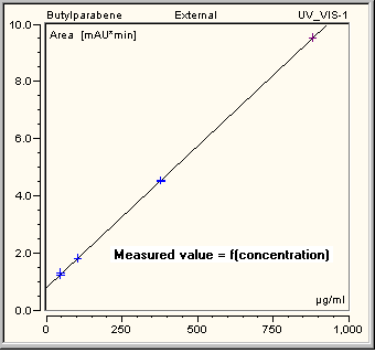
Normally, calibration curves are fitted using normal regression analysis, in which the known amount (or concentration) of the analyte is treated as the independent variable (x) and the corresponding response (peak area or peak height) is treated as the dependent variable (y):

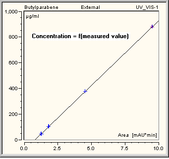
Many legacy data systems use inverted curve fitting, which treats the response as if it were the independent variable (x), and amount as if it were the dependent variable (y):

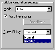
You can select the Inverted curve fitting option on the General tab page:

Although standard statistical theory does not support inverted curve fitting, it was often taken because it makes amounts of analytes in unknowns easier to calculate when quadratic and cubic calibration functions are used. With linear regression, the differences between normal and inverted curve fitting are usually small, but the differences can be significant with higher-order polynomials. In a few applications, most notably the determination of ammonium by suppressed conductivity detection, a better fit to the empirical data may actually be achieved using inverted curve fitting.
To provide consistency of results for customers migrating from legacy systems, and to satisfy users of special applications, Chromeleon supports inverted curve fitting via an option in the General tab page of the QNT Editor. Methods imported from PeakNet 5 default to using inverted curve fitting, the approach used by PeakNet 5. Normal curve fitting remains the default setting for new methods created in Chromeleon.
![]() Caution:
Caution:
It is the user's responsibility to decide whether inverted curve fitting is sensible for their application.
If you select Inverted, the dependent and independent variables are inverted. Thus, different values are usually obtained for the following variables:
Peak Results Category
Amount (concentration or amount)
Amount Deviation (deviation from the expected concentration or amount)
Concentration (concentration, if Amount is really an amount)
Relative Amount (relative concentration or amount)
Group Amount (concentration or amount of a group)
Peak Calibration Category
Offset c0 (intersection with the y-axis)
Curve c2 (curvature)
RF Value (1/slope)
Calibration Point X
Calibration Point Y
Evaluation of Cal.Function for X ()
Residual for Calibration Point X
Upper Confidence Limit (upper limit for the Confidence Interval)
Lower Confidence Limit (lower limit for the confidence interval)