INDEX

Description

INDEX returns the contents of a cell from a specified range.

Syntax

INDEX ( reference [, row] [, column] [, range_number] )

Parameter	Description
reference	A reference to one or more ranges. If reference specifies more than one range, separate each reference with the list separator and enclose reference in parentheses. For example, (A1:C6, B7:E14, F4). If each range in reference contains only one row or column, you can omit the row or column argument. For example, if reference is A1:A15, you can omit the column argument INDEX(A1:A15, 3,, 1).
Row	The row number in reference from which to return data.
Column	Column number in reference from which to return data.
Range_number	Specifies the range from which data is returned if reference contains more than one range. For example, if reference is (A1:A10, B1:B5, D14:E23), A1:A10 is range_number 1, B1:B5 is range_number 2, and D14:E23 is range_number 3.

Remarks

If row, column, and range_number do not point to a cell within reference, #REF! is returned. If row and column are omitted, INDEX returns the range in reference specified by range_number.

Examples

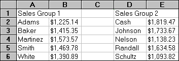
The following examples use this worksheet.

This function returns $1415.35:

INDEX(A2:B6, 2, 2)

This function returns $1634.58:

INDEX((A2:B6, D2:E6), 4, 2, 2)

Note:

If an Invalid formula syntax warning appears, check whether the comma is set as the list separator in your regional settings on the Windows Control Panel. If a different character is set as the list separator, use this character in the above examples in place of the comma. (Windows XP: Access the Windows Control Panel and select Regional and Language Options. On the Regional Options tab page, click Customize. On the Numbers tab page, check which character is the default list separator on your computer. Use this character in the above examples instead of the comma.

Also, see